Quick and pretty frequency tables with ivo_table_gt

Background

R has some great packages for creating nice-looking tables. Packages like gt and flextable allow the user to create a wide range of tables, with lots of flexibility in how these are presented and formatted. The downside to these Swiss army knife-style packages is that simple tasks, like creating a frequency table, require a lot of typing. Enter ivo.table, a package for creating great-looking frequency tables and contingency tables without any hassle.

The package offers two functions for creating tables: ivo_table, which uses the flextable framework, and ivo_table_gt which uses the gt framework. This vignette contains examples using the latter.

A first example

Let’s look at some examples using the penguins data from the palmerpenguins package. Say that we want to create a contingency table showing the counts of the categorical variables species, sex, and island. We can use ftable along with dplyr’s select:

library(dplyr)
#> 
#> Attaching package: 'dplyr'
#> The following objects are masked from 'package:stats':
#> 
#>     filter, lag
#> The following objects are masked from 'package:base':
#> 
#>     intersect, setdiff, setequal, union
library(palmerpenguins)

penguins |> select(species, sex, island) |> ftable()
#>                  island Biscoe Dream Torgersen
#> species   sex                                 
#> Adelie    female            22    27        24
#>           male              22    28        23
#> Chinstrap female             0    34         0
#>           male               0    34         0
#> Gentoo    female            58     0         0
#>           male              61     0         0

While informative, the formatting isn’t great, and it’s not something that we can easily export to a report or presentation.

ivo.table uses the same syntax, but with ivo_table_gt instead of ftable:

library(ivo.table)

penguins |> select(species, sex, island) |> ivo_table_gt()

	species
	Adelie	Chinstrap	Gentoo
female
Biscoe	22	0	58
Dream	27	34	0
Torgersen	24	0	0
male
Biscoe	22	0	61
Dream	28	34	0
Torgersen	23	0	0
(Missing)
Biscoe	0	0	5
Dream	1	0	0
Torgersen	5	0	0

You can add row and column sums:

penguins |>
  select(species, sex, island) |>
  ivo_table_gt(sums = c("cols", "rows"))

	species			Total
	Adelie	Chinstrap	Gentoo
female
Biscoe	22	0	58	80
Dream	27	34	0	61
Torgersen	24	0	0	24
Total	73	34	58	165
male
Biscoe	22	0	61	83
Dream	28	34	0	62
Torgersen	23	0	0	23
Total	73	34	61	168
(Missing)
Biscoe	0	0	5	5
Dream	1	0	0	1
Torgersen	5	0	0	5
Total	6	0	5	11

Changing the appearance of your tables

You can customise the look of your ivo_table_gt table using styling arguments and gt functions. You can change the colours and fonts used, highlight columns, rows or cells, make columns bold, and more. Let’s look at some examples.

Change the font to Courier, use red instead of green, and make the names in the sex column bold:

library(gt)
penguins |>
  select(species, sex, island) |>
  ivo_table_gt(color = "red",
               font_name = "Courier") |> 
  tab_style(style = list(cell_text(weight = "bold")),
                locations = cells_stub())

	species
	Adelie	Chinstrap	Gentoo
female
Biscoe	22	0	58
Dream	27	34	0
Torgersen	24	0	0
male
Biscoe	22	0	61
Dream	28	34	0
Torgersen	23	0	0
(Missing)
Biscoe	0	0	5
Dream	1	0	0
Torgersen	5	0	0

Add a caption and highlight the cell on the fourth row of the third column:

penguins |>
  select(species, sex, island) |>
  ivo_table_gt(caption = "A table with penguins in it") |> 
    tab_style(style = list(cell_fill(color = "darkgreen")),
                locations = cells_body(columns = 5, rows = 4))

A table with penguins in it
	species
	Adelie	Chinstrap	Gentoo
female
Biscoe	22	0	58
Dream	27	34	0
Torgersen	24	0	0
male
Biscoe	22	0	61
Dream	28	34	0
Torgersen	23	0	0
(Missing)
Biscoe	0	0	5
Dream	1	0	0
Torgersen	5	0	0

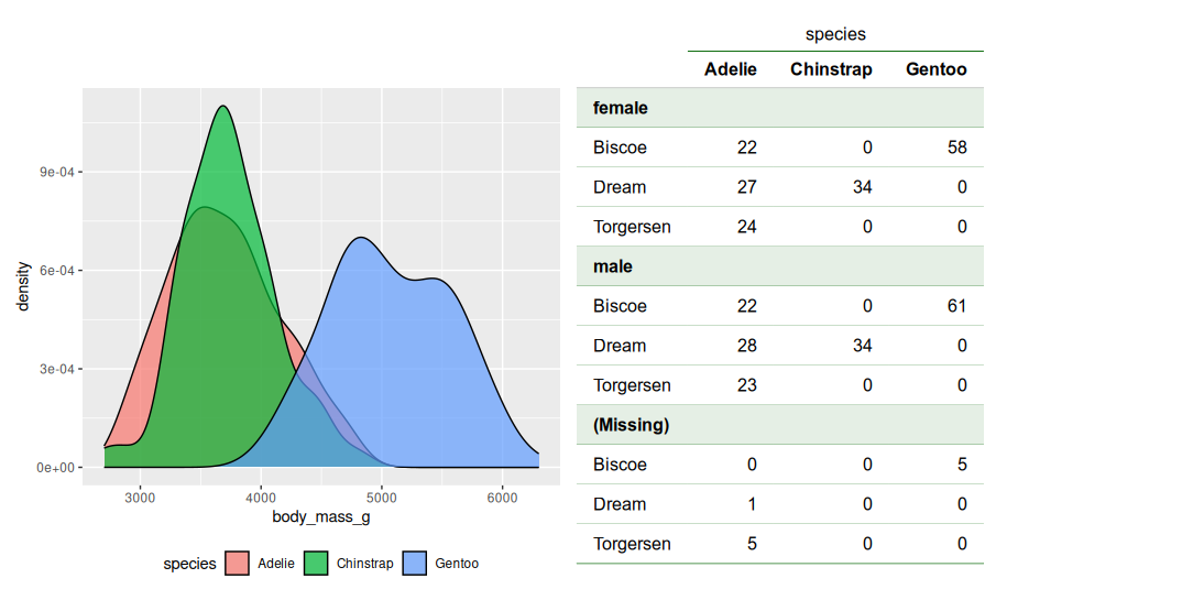
ivo_table_gt returns a gt object, meaning that all functions used to style gt tables can be used. You can also paste ggplot2 plots and tables together using patchwork:

library(ggplot2)
library(patchwork)

penguins_plot <- ggplot(penguins, aes(body_mass_g, fill = species)) +
                    geom_density(alpha = 0.7) +
                    theme(legend.position = "bottom")

penguins_table <- penguins |>
                    select(species, sex, island) |>
                    ivo_table_gt()

penguins_plot + penguins_table